第十五讲：子空间投影

从 $R^{2}$ 空间讲起，有向量 $a, b$ ，做 $b$ 在 $a$ 上的投影 $p$ ，如图：

python

%matplotlib inline
import matplotlib.pyplot as plt
import numpy as np
import pandas as pd

plt.style.use("seaborn-dark-palette")

fig = plt.figure()
plt.axis('equal')
plt.axis([-7, 7, -6, 6])
plt.arrow(-4, -1, 8, 2, head_width=0.3, head_length=0.5, color='r', length_includes_head=True)
plt.arrow(0, 0, 2, 4, head_width=0.3, head_length=0.5, color='b', length_includes_head=True)
plt.arrow(0, 0, 48/17, 12/17, head_width=0.3, head_length=0.5, color='gray', length_includes_head=True)
plt.arrow(48/17, 12/17, 2-48/17, 4-12/17, head_width=0.3, head_length=0.5, color='g', length_includes_head=True)
# plt.plot([48/17], [12/17], 'o')
# y=1/4x
# y=-4x+12
# x=48/17
# y=12/17
plt.annotate('b', xy=(1, 2), xytext=(-30, 15), textcoords='offset points', size=20, arrowprops=dict(arrowstyle="->"))
plt.annotate('a', xy=(-1, -0.25), xytext=(15, -30), textcoords='offset points', size=20, arrowprops=dict(arrowstyle="->"))
plt.annotate('e=b-p', xy=(2.5, 2), xytext=(30, 0), textcoords='offset points', size=20, arrowprops=dict(arrowstyle="->"))
plt.annotate('p=xa', xy=(2, 0.5), xytext=(-20, -40), textcoords='offset points', size=20, arrowprops=dict(arrowstyle="->"))
plt.grid()

%matplotlib inline
import matplotlib.pyplot as plt
import numpy as np
import pandas as pd

plt.style.use("seaborn-dark-palette")

fig = plt.figure()
plt.axis('equal')
plt.axis([-7, 7, -6, 6])
plt.arrow(-4, -1, 8, 2, head_width=0.3, head_length=0.5, color='r', length_includes_head=True)
plt.arrow(0, 0, 2, 4, head_width=0.3, head_length=0.5, color='b', length_includes_head=True)
plt.arrow(0, 0, 48/17, 12/17, head_width=0.3, head_length=0.5, color='gray', length_includes_head=True)
plt.arrow(48/17, 12/17, 2-48/17, 4-12/17, head_width=0.3, head_length=0.5, color='g', length_includes_head=True)
# plt.plot([48/17], [12/17], 'o')
# y=1/4x
# y=-4x+12
# x=48/17
# y=12/17
plt.annotate('b', xy=(1, 2), xytext=(-30, 15), textcoords='offset points', size=20, arrowprops=dict(arrowstyle="->"))
plt.annotate('a', xy=(-1, -0.25), xytext=(15, -30), textcoords='offset points', size=20, arrowprops=dict(arrowstyle="->"))
plt.annotate('e=b-p', xy=(2.5, 2), xytext=(30, 0), textcoords='offset points', size=20, arrowprops=dict(arrowstyle="->"))
plt.annotate('p=xa', xy=(2, 0.5), xytext=(-20, -40), textcoords='offset points', size=20, arrowprops=dict(arrowstyle="->"))
plt.grid()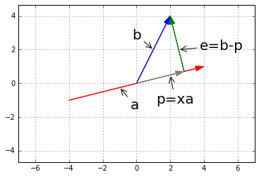

png

python

plt.close(fig)

plt.close(fig)

从图中我们知道，向量 $e$ 就像是向量 $b, p$ 之间的误差， $e = b - p, e ⊥ p$ 。 $p$ 在 $a$ 上，有 $\underset{―}{p = a x}$ 。

所以有 $a^{T} e = a^{T} (b - p) = a^{T} (b - a x) = 0$ 。关于正交的最重要的方程：

a^{T} (b - x a) = 0 \underset{―}{x a^{T} a = a^{T} b} \underset{―}{x = \frac{a^{T} b}{a^{T} a}} p = a \frac{a^{T} b}{a^{T} a}

从上面的式子可以看出，如果将 $b$ 变为 $2 b$ 则 $p$ 也会翻倍，如果将 $a$ 变为 $2 a$ 则 $p$ 不变。

设投影矩阵为 $P$ ，则可以说投影矩阵作用与某个向量后，得到其投影向量， $p r o j e c t i o n_{p} = P b$ 。

易看出 $\underset{―}{P = \frac{a a^{T}}{a^{T} a}}$ ，若 $a$ 是 $n$ 维列向量，则 $P$ 是一个 $n \times n$ 矩阵。

观察投影矩阵 $P$ 的列空间， $C (P)$ 是一条通过 $a$ 的直线，而 $r a n k (P) = 1$ （一列乘以一行： $a a^{T}$ ，而这一列向量 $a$ 是该矩阵的基）。

投影矩阵的性质：

$\underset{―}{P = P^{T}}$ ，投影矩阵是一个对称矩阵。
如果对一个向量做两次投影，即 $P P b$ ，则其结果仍然与 $P b$ 相同，也就是 $\underset{―}{P^{2} = P}$ 。

为什么我们需要投影？因为就像上一讲中提到的，有些时候 $A x = b$ 无解，我们只能求出最接近的那个解。

$A x$ 总是在 $A$ 的列空间中，而 $b$ 却不一定，这是问题所在，所以我们可以将 $b$ 变为 $A$ 的列空间中最接近的那个向量，即将无解的 $A x = b$ 变为求有解的 $A \hat{x} = p$ （ $p$ 是 $b$ 在 $A$ 的列空间中的投影， $\hat{x}$ 不再是那个不存在的 $x$ ，而是最接近的解）。

现在来看 $R^{3}$ 中的情形，将向量 $b$ 投影在平面 $A$ 上。同样的， $p$ 是向量 $b$ 在平面 $A$ 上的投影， $e$ 是垂直于平面 $A$ 的向量，即 $b$ 在平面 $A$ 法方向的分量。设平面 $A$ 的一组基为 $a_{1}, a_{2}$ ，则投影向量 $p = \hat{x_{1}} a_{1} + \hat{x_{2}} a_{2}$ ，我们更倾向于写作 $p = A \hat{x}$ ，这里如果我们求出 $\hat{x}$ ，则该解就是无解方程组最近似的解。

现在问题的关键在于找 $e = b - A \hat{x}$ ，使它垂直于平面，因此我们得到两个方程 ${\begin{cases} a_{1}^{T} (b - A \hat{x}) = 0 \\ a_{2}^{T} (b - A \hat{x}) = 0 \end{cases}$ ，将方程组写成矩阵形式 $[\begin{matrix} a_{1}^{T} \\ a_{2}^{T} \end{matrix}] (b - A \hat{x}) = [\begin{matrix} 0 \\ 0 \end{matrix}]$ ，即 $A^{T} (b - A \hat{x}) = 0$ 。

比较该方程与 $R^{2}$ 中的投影方程，发现只是向量 $a$ 变为矩阵 $A$ 而已，本质上就是 $A^{T} e = 0$ 。所以， $e$ 在 $A^{T}$ 的零空间中（ $e \in N (A^{T})$ ），从前面几讲我们知道，左零空间 $⊥$ 列空间，则有 $e ⊥ C (A)$ ，与我们设想的一致。

再化简方程得 $A^{T} A x = A^{T} b$ ，比较在 $R^{2}$ 中的情形， $a^{T} a$ 是一个数字而 $A^{T} A$ 是一个 $n$ 阶方阵，而解出的 $x$ 可以看做两个数字的比值。现在在 $R^{3}$ 中，我们需要再次考虑：什么是 $\hat{x}$ ？投影是什么？投影矩阵又是什么？

第一个问题： $\hat{x} = (A^{T} A)^{- 1} A^{T} b$ ；
第二个问题： $p = A \hat{x} = \underset{―}{A (A^{T} A)^{- 1} A^{T}} b$ ，回忆在 $R^{2}$ 中的情形，下划线部分就是原来的 $\frac{a a^{T}}{a^{T} a}$ ；
第三个问题：易看出投影矩阵就是下划线部分 $P = A (A^{T} A)^{- 1} A^{T}$ 。

这里还需要注意一个问题， $P = A (A^{T} A)^{- 1} A^{T}$ 是不能继续化简为 $P = A A^{- 1} (A^{T})^{- 1} A^{T} = I$ 的，因为这里的 $A$ 并不是一个可逆方阵。也可以换一种思路，如果 $A$ 是一个 $n$ 阶可逆方阵，则 $A$ 的列空间是整个 $R^{n}$ 空间，于是 $b$ 在 $R^{n}$ 上的投影矩阵确实变为了 $I$ ，因为 $b$ 已经在空间中了，其投影不再改变。

再来看投影矩阵 $P$ 的性质：

$P = P^{T}$ ：有 ${[A (A^{T} A)^{- 1} A^{T}]}^{T} = A {[(A^{T} A)^{- 1}]}^{T} A^{T}$ ，而 $(A^{T} A)$ 是对称的，所以其逆也是对称的，所以有 $A ((A^{T} A)^{- 1})^{T} A^{T} = A (A^{T} A)^{- 1} A^{T}$ ，得证。
$P^{2} = P$ ：有 $[A (A^{T} A)^{- 1} A^{T}] [A (A^{T} A)^{- 1} A^{T}] = A (A^{T} A)^{- 1} [(A^{T} A) (A^{T} A)^{- 1}] A^{T} = A (A^{T} A)^{- 1} A^{T}$ ，得证。

最小二乘法

接下看看投影的经典应用案例：最小二乘法拟合直线（least squares fitting by a line）。

我们需要找到距离图中三个点 $(1, 1), (2, 2), (3, 2)$ 偏差最小的直线： $b = C + D t$ 。

python

plt.style.use("seaborn-dark-palette")

fig = plt.figure()
plt.axis('equal')
plt.axis([-1, 4, -1, 3])
plt.axhline(y=0, c='black', lw='2')
plt.axvline(x=0, c='black', lw='2')

plt.plot(1, 1, 'o', c='r')
plt.plot(2, 2, 'o', c='r')
plt.plot(3, 2, 'o', c='r')

plt.annotate('(1, 1)', xy=(1, 1), xytext=(-40, 20), textcoords='offset points', size=14, arrowprops=dict(arrowstyle="->"))
plt.annotate('(2, 2)', xy=(2, 2), xytext=(-60, -5), textcoords='offset points', size=14, arrowprops=dict(arrowstyle="->"))
plt.annotate('(3, 2)', xy=(3, 2), xytext=(-18, 20), textcoords='offset points', size=14, arrowprops=dict(arrowstyle="->"))

plt.grid()

plt.style.use("seaborn-dark-palette")

fig = plt.figure()
plt.axis('equal')
plt.axis([-1, 4, -1, 3])
plt.axhline(y=0, c='black', lw='2')
plt.axvline(x=0, c='black', lw='2')

plt.plot(1, 1, 'o', c='r')
plt.plot(2, 2, 'o', c='r')
plt.plot(3, 2, 'o', c='r')

plt.annotate('(1, 1)', xy=(1, 1), xytext=(-40, 20), textcoords='offset points', size=14, arrowprops=dict(arrowstyle="->"))
plt.annotate('(2, 2)', xy=(2, 2), xytext=(-60, -5), textcoords='offset points', size=14, arrowprops=dict(arrowstyle="->"))
plt.annotate('(3, 2)', xy=(3, 2), xytext=(-18, 20), textcoords='offset points', size=14, arrowprops=dict(arrowstyle="->"))

plt.grid()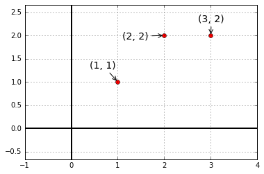

png

python

plt.close(fig)

plt.close(fig)

根据条件可以得到方程组 ${\begin{cases} C + D & = 1 \\ C + 2 D & = 2 \\ C + 3 D & = 2 \end{cases}$ ，写作矩阵形式 $[\begin{matrix} 1 & 1 \\ 1 & 2 \\ 1 & 3 \end{matrix}] [\begin{matrix} C \\ D \end{matrix}] = [\begin{matrix} 1 \\ 2 \\ 2 \end{matrix}]$ ，也就是我们的 $A x = b$ ，很明显方程组无解。但是 $A^{T} A \hat{x} = A^{T} b$ 有解，于是我们将原是两边同时乘以 $A^{T}$ 后得到的新方程组是有解的， $A^{T} A \hat{x} = A^{T} b$ 也是最小二乘法的核心方程。

下一讲将进行最小二乘法的验算。

第十五讲：子空间投影 ​

最小二乘法 ​

第十五讲：子空间投影

最小二乘法