第十六讲：投影矩阵和最小二乘

上一讲中，我们知道了投影矩阵 $P = A (A^{T} A)^{- 1} A^{T}$ ， $P b$ 将会把向量投影在 $A$ 的列空间中。

举两个极端的例子：

如果 $b \in C (A)$ ，则 $P b = b$ ；
如果 $b ⊥ C (A)$ ，则 $P b = 0$ 。

一般情况下， $b$ 将会有一个垂直于 $A$ 的分量，有一个在 $A$ 列空间中的分量，投影的作用就是去掉垂直分量而保留列空间中的分量。

在第一个极端情况中，如果 $b \in C (A)$ 则有 $b = A x$ 。带入投影矩阵 $p = P b = A (A^{T} A)^{- 1} A^{T} A x = A x$ ，得证。

在第二个极端情况中，如果 $b ⊥ C (A)$ 则有 $b \in N (A^{T})$ ，即 $A^{T} b = 0$ 。则 $p = P b = A (A^{T} A)^{- 1} A^{T} b = 0$ ，得证。

向量 $b$ 投影后，有 $b = e + p, p = P b, e = (I - P) b$ ，这里的 $p$ 是 $b$ 在 $C (A)$ 中的分量，而 $e$ 是 $b$ 在 $N (A^{T})$ 中的分量。

回到上一讲最后提到的例题：

我们需要找到距离图中三个点 $(1, 1), (2, 2), (3, 2)$ 偏差最小的直线： $y = C + D t$ 。

python

%matplotlib inline
import matplotlib.pyplot as plt
from sklearn import linear_model
import numpy as np
import pandas as pd
import seaborn as sns

x = np.array([1, 2, 3]).reshape((-1,1))
y = np.array([1, 2, 2]).reshape((-1,1))
predict_line = np.array([-1, 4]).reshape((-1,1))

regr = linear_model.LinearRegression()
regr.fit(x, y)
ey = regr.predict(x)

fig = plt.figure()
plt.axis('equal')
plt.axhline(y=0, c='black')
plt.axvline(x=0, c='black')

plt.scatter(x, y, c='r')
plt.scatter(x, regr.predict(x), s=20, c='b')
plt.plot(predict_line, regr.predict(predict_line), c='g', lw='1')
[ plt.plot([x[i], x[i]], [y[i], ey[i]], 'r', lw='1') for i in range(len(x))]

plt.annotate('(1, 1)', xy=(1, 1), xytext=(-15, -30), textcoords='offset points', size=14, arrowprops=dict(arrowstyle="->"))
plt.annotate('(2, 2)', xy=(2, 2), xytext=(-60, -5), textcoords='offset points', size=14, arrowprops=dict(arrowstyle="->"))
plt.annotate('(3, 2)', xy=(3, 2), xytext=(-15, -30), textcoords='offset points', size=14, arrowprops=dict(arrowstyle="->"))

plt.annotate('$e_1$', color='r', xy=(1, 1), xytext=(0, 2), textcoords='offset points', size=20)
plt.annotate('$e_2$', color='r', xy=(2, 2), xytext=(0, -15), textcoords='offset points', size=20)
plt.annotate('$e_3$', color='r', xy=(3, 2), xytext=(0, 1), textcoords='offset points', size=20)

plt.annotate('$p_1$', xy=(1, 7/6), color='b', xytext=(-7, 30), textcoords='offset points', size=14, arrowprops=dict(arrowstyle="->"))
plt.annotate('$p_2$', xy=(2, 5/3), color='b', xytext=(-7, -30), textcoords='offset points', size=14, arrowprops=dict(arrowstyle="->"))
plt.annotate('$p_3$', xy=(3, 13/6), color='b', xytext=(-7, 30), textcoords='offset points', size=14, arrowprops=dict(arrowstyle="->"))
plt.draw()

%matplotlib inline
import matplotlib.pyplot as plt
from sklearn import linear_model
import numpy as np
import pandas as pd
import seaborn as sns

x = np.array([1, 2, 3]).reshape((-1,1))
y = np.array([1, 2, 2]).reshape((-1,1))
predict_line = np.array([-1, 4]).reshape((-1,1))

regr = linear_model.LinearRegression()
regr.fit(x, y)
ey = regr.predict(x)

fig = plt.figure()
plt.axis('equal')
plt.axhline(y=0, c='black')
plt.axvline(x=0, c='black')

plt.scatter(x, y, c='r')
plt.scatter(x, regr.predict(x), s=20, c='b')
plt.plot(predict_line, regr.predict(predict_line), c='g', lw='1')
[ plt.plot([x[i], x[i]], [y[i], ey[i]], 'r', lw='1') for i in range(len(x))]

plt.annotate('(1, 1)', xy=(1, 1), xytext=(-15, -30), textcoords='offset points', size=14, arrowprops=dict(arrowstyle="->"))
plt.annotate('(2, 2)', xy=(2, 2), xytext=(-60, -5), textcoords='offset points', size=14, arrowprops=dict(arrowstyle="->"))
plt.annotate('(3, 2)', xy=(3, 2), xytext=(-15, -30), textcoords='offset points', size=14, arrowprops=dict(arrowstyle="->"))

plt.annotate('$e_1$', color='r', xy=(1, 1), xytext=(0, 2), textcoords='offset points', size=20)
plt.annotate('$e_2$', color='r', xy=(2, 2), xytext=(0, -15), textcoords='offset points', size=20)
plt.annotate('$e_3$', color='r', xy=(3, 2), xytext=(0, 1), textcoords='offset points', size=20)

plt.annotate('$p_1$', xy=(1, 7/6), color='b', xytext=(-7, 30), textcoords='offset points', size=14, arrowprops=dict(arrowstyle="->"))
plt.annotate('$p_2$', xy=(2, 5/3), color='b', xytext=(-7, -30), textcoords='offset points', size=14, arrowprops=dict(arrowstyle="->"))
plt.annotate('$p_3$', xy=(3, 13/6), color='b', xytext=(-7, 30), textcoords='offset points', size=14, arrowprops=dict(arrowstyle="->"))
plt.draw()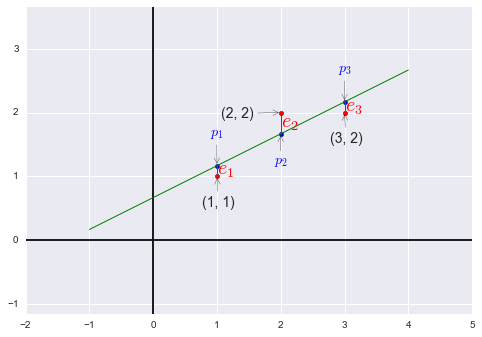

png

python

plt.close(fig)

plt.close(fig)

根据条件可以得到方程组 ${\begin{cases} C + D & = 1 \\ C + 2 D & = 2 \\ C + 3 D & = 2 \end{cases}$ ，写作矩阵形式 $[\begin{matrix} 1 & 1 \\ 1 & 2 \\ 1 & 3 \end{matrix}] [\begin{matrix} C \\ D \end{matrix}] = [\begin{matrix} 1 \\ 2 \\ 2 \end{matrix}]$ ，也就是我们的 $A x = b$ ，很明显方程组无解。

我们需要在 $b$ 的三个分量上都增加某个误差 $e$ ，使得三点能够共线，同时使得 $e_{1}^{2} + e_{2}^{2} + e_{3}^{2}$ 最小，找到拥有最小平方和的解（即最小二乘），即 ${‖ A x - b ‖}^{2} = {‖ e ‖}^{2}$ 最小。此时向量 $b$ 变为向量 $p = [\begin{matrix} p_{1} \\ p_{2} \\ p_{3} \end{matrix}]$ （在方程组有解的情况下， $A x - b = 0$ ，即 $b$ 在 $A$ 的列空间中，误差 $e$ 为零。）我们现在做的运算也称作线性回归（linear regression），使用误差的平方和作为测量总误差的标准。

注：如果有另一个点，如 $(0, 100)$ ，在本例中该点明显距离别的点很远，最小二乘将很容易被离群的点影响，通常使用最小二乘时会去掉明显离群的点。

现在我们尝试解出 $\hat{x} = [\begin{matrix} \hat{C} \\ \hat{D} \end{matrix}]$ 与 $p = [\begin{matrix} p_{1} \\ p_{2} \\ p_{3} \end{matrix}]$ 。

A^{T} A \hat{x} = A^{T} b A^{T} A = [\begin{matrix} 3 & 6 \\ 6 & 14 \end{matrix}] A^{T} b = [\begin{matrix} 5 \\ 11 \end{matrix}] [\begin{matrix} 3 & 6 \\ 6 & 14 \end{matrix}] [\begin{matrix} \hat{C} \\ \hat{D} \end{matrix}] = [\begin{matrix} 5 \\ 11 \end{matrix}]

写作方程形式为 ${\begin{cases} 3 \hat{C} + 16 \hat{D} & = 5 \\ 6 \hat{C} + 14 \hat{D} & = 11 \end{cases}$ ，也称作正规方程组（normal equations）。

回顾前面提到的“使得误差最小”的条件， $e_{1}^{2} + e_{2}^{2} + e_{3}^{2} = (C + D - 1)^{2} + (C + 2 D - 2)^{2} + (C + 3 D - 2)^{2}$ ，使该式取最小值，如果使用微积分方法，则需要对该式的两个变量 $C, D$ 分别求偏导数，再令求得的偏导式为零即可，正是我们刚才求得的正规方程组。（正规方程组中的第一个方程是对 $C$ 求偏导的结果，第二个方程式对 $D$ 求偏导的结果，无论使用哪一种方法都会得到这个方程组。）

解方程得 $\hat{C} = \frac{2}{3}, \hat{D} = \frac{1}{2}$ ，则“最佳直线”为 $y = \frac{2}{3} + \frac{1}{2} t$ ，带回原方程组解得 $p_{1} = \frac{7}{6}, p_{2} = \frac{5}{3}, p_{3} = \frac{13}{6}$ ，即 $e_{1} = - \frac{1}{6}, e_{2} = \frac{1}{3}, e_{3} = - \frac{1}{6}$

于是我们得到 $p = [\begin{matrix} \frac{7}{6} \\ \frac{5}{3} \\ \frac{13}{6} \end{matrix}], e = [\begin{matrix} - \frac{1}{6} \\ \frac{1}{3} \\ - \frac{1}{6} \end{matrix}]$ ，易看出 $b = p + e$ ，同时我们发现 $p \cdot e = 0$ 即 $p ⊥ e$ 。

误差向量 $e$ 不仅垂直于投影向量 $p$ ，它同时垂直于列空间，如 $[\begin{matrix} 1 \\ 1 \\ 1 \end{matrix}], [\begin{matrix} 1 \\ 2 \\ 3 \end{matrix}]$ 。

接下来我们观察 $A^{T} A$ ，如果 $A$ 的各列线性无关，求证 $A^{T} A$ 是可逆矩阵。

先假设 $A^{T} A x = 0$ ，两边同时乘以 $x^{T}$ 有 $x^{T} A^{T} A x = 0$ ，即 $(A x)^{T} (A x) = 0$ 。一个矩阵乘其转置结果为零，则这个矩阵也必须为零（ $(A x)^{T} (A x)$ 相当于 $A x$ 长度的平方）。则 $A x = 0$ ，结合题设中的“ $A$ 的各列线性无关”，可知 $x = 0$ ，也就是 $A^{T} A$ 的零空间中有且只有零向量，得证。

我们再来看一种线性无关的特殊情况：互相垂直的单位向量一定是线性无关的。

比如 $[\begin{matrix} 1 \\ 0 \\ 0 \end{matrix}] [\begin{matrix} 0 \\ 1 \\ 0 \end{matrix}] [\begin{matrix} 0 \\ 0 \\ 1 \end{matrix}]$ ，这三个正交单位向量也称作标准正交向量组（orthonormal vectors）。
另一个例子 $[\begin{matrix} \cos θ \\ \sin θ \end{matrix}] [\begin{matrix} - \sin θ \\ \cos θ \end{matrix}]$

下一讲研究标准正交向量组。

第十六讲：投影矩阵和最小二乘 ​

第十六讲：投影矩阵和最小二乘